Variogram Model > Variogram Theory Models

Variogram Theory Models

Between the separate-vector values of sample location and estimated location, there may be some variogram values which we need but we cannot obtain exist. In order to obtain an accurate Kriging matrix, we have to calculate the variogram value of a possible separate vector through some transformation models. In fact, the γ (h) value of variogram models is unknown. We have to estimate the γ (h) value with samples from an effective space and calculate a series of γ(h) values according to different h values. To date, the popular models in statistics are the Spherical Model, Exponential Model, and Gaussian Model. First of all, we have to understand some features of the models.

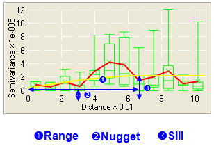
•Range & Sill

When you establish a variogram model, you may observe that the curve in the graph climbs for a certain distance and then becomes parallel to the X-axis and extends to the right side. This climbing distance is called “Range”. There are correlations between samples in this “Range”. On the contrary, there are no correlations between samples beyond this “Range”. The values the “Range” can reach, meaning that the Y-axis to which the X-axis of “range” corresponds, is “Sill”. Partial Sill is the differences of Sill minus Nugget Effect.

•Nugget Effect

Theoretically, if the measuring distance between 2 points is 0 (Lag=0), then its semivariance should be 0 as well. However, practically, there are still some “infinitesimal” distances between sample points. Therefore, 0 will not be reached, and this is called “Nugget Effect.”

Nugget Effect may be caused by the measurement errors or by the less distance change between point data than the microscale variations of samples.