
Isotropy and Anisotropy
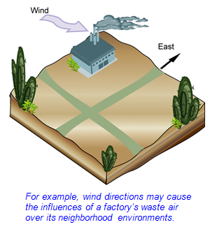
In geostatistical analysis, there are two directional influences: one is the trend of a whole region, and the other one is the anisotropic settings in the semivariogram models. The whole-region trend could be estimated through some mathematical estimation models, such as polynomial, and could eliminate influences during the process of geostatistical analysis.
With regard to the isotropy and anisotropy, geostatistical analysis employ the variograms to present the correlations of spatial variability. A variogram model is a distance function. If the variogram of a spatial variance is merely a distance function and the variability does not vary along with spatial directions, this is called “Isotropy”. If the variability varies along with spatial directions, this is called “Anisotropy”. In other words, the anisotropic variogram model is the function of “distance” and “direction”, and the equation could be presented as follows:
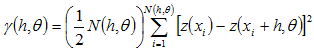
θ:the angle along Point ![]() and
and![]()
![]() :pairs of samples with interval “h" in the angles along point
:pairs of samples with interval “h" in the angles along point ![]() and
and![]() .
.
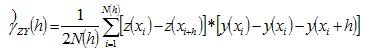
If there are 2 regionalized variables “z” and “y”, the joint variogram could be obtained via:
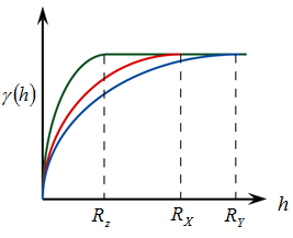
General speaking, the procedures of distinguishing between isotropy and anisotropy are the same. We can fit a variogram model along all the directions and then obtain different variograms along with different directions. Once we obtain the values of Still, Range, Nugget Effect from all variograms, we can determine if the spatial data is isotropic or anisotropic. If the values of Still, Range, Nugget Effect from the variogram along with all directions are all the same, then it is isotropic; otherwise, it is the anisotropic.
Anisotropy, according to its different structures, could be divided into Geometric Anisotropy, Zonal Anisotropy, and Mixed Anisotropy.
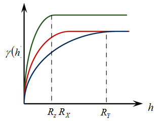
The Sill value of the Geometric Anisotropic variogram only vary along with distances, but not along with directions. In other words, when the distances between samples in various spatial angles are the same, their Sill is the same, but their ranges may vary along with different angles. The direction having biggest range is the direction of variogram. This range is called “Major Range”, and this variogram is called Directional Variogram. The smallest range is called “Minor Range”. If we draw the spatial ranges of all angles on a rose diagram, the shape is an ellipse.
|
The Sill value of the Zonal Anisotropic variogram does not only vary along with all distances, but also varies along with all directions. In other words, when the distances between samples in any spatial angles are the same, their Sill values are not the same, and their ranges also vary along with different angles. Zonal Anisotropic variogram model consists of 2 or more than 2 anisotropic variograms. Natural phenomena usually do not have this kind of anisotropy.
|
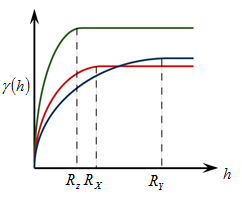
The Mixed Anisotropiy is a mix of the Geometric Anisotropy and Zonal Anisotropy . Its Sill values and ranges vary along with all directions. Natural phenomena usually have this kind of spatial variability. For example, geological changes usually have a bigger effective range in the horizon direction than in the vertical direction, and changes in the vertical driection have a bigger range than in the horizon direction.
|
©2017 Supergeo Technologies Inc. All rights reserved.